We created this article to present a solution designed to handle the distribution of the computation tasks that arise when we run deep learning experiments that require heavy processing to generate data during the training process. It shows a practical case study for the usual broker pattern, and gives an example of how it is possible to painlessly deploy with Docker the different components of the system’s stack. In our case, we mean:

• a RabbitMQ server hosting the job queues
• a manager server to administer computation sessions
• swarms of workers to handle the computation tasks associated with each experiment
• a program that controls the health of the clusters of workers and that adapts the publish rate of the tasks in real-time.

The application layer, used by the manager and worker components, has been developed in python using the framework Celery. Other technologies involved are:

• Docker, docker-compose, docker swarm, docker stack
• Flask (for the manager server), Tornado (for asynchronous networking in the health controller)
• Joblib to cache the results of the tasks

Introducing the problem

At Deezer’s Research and Development team, a large part of our activities consists in designing deep learning experiments, and training models able to generate knowledge on our track database. Examples of such system are:

Royo-Letelier, Jimena, Romain Hennequin, and Manuel Moussallam. “Mirex 2015 music/speech classification.” Music Inform. Retrieval Evaluation eXchange (MIREX) (2015).

Hennequin, Romain, Jimena Royo-Letelier, and Manuel Moussallam. “Codec independent lossy audio compression detection.” Acoustics, Speech and Signal Processing (ICASSP), 2017 IEEE International Conference on. IEEE, 2017.

Below is shown a typical representation of an experiment.

In our case study, the data generation pipeline is run on CPU, while the training is performed on GPU. The data generation takes its source from a dataset specific to the experiment, as represented by the circle in the figure above.

When in production, these systems run permanently, analyzing everything that is added to the catalog, and exporting information that will serve various purposes, like fueling up our recommendation systems. However, bringing such systems to production takes time, and tremendous research efforts are invested into the design of the experiment that will produce the best results. Training a model is a very lengthy process, especially when the number of parameters is high and the size of the dataset large. Another factor that can increase the training time is the generation of a the data that goes into the system. Let’s start by taking a look at what the features are, to make this statement clearer.

What are features all about?

In a lot of experiments, akin to those involving images, raw data is directly fed into the network, with possibly light preprocessing. In this situation, the time taken to generate new batches to train the model on is effectively negligible compared to the time taken by the training pass. This is even more so when the whole database can fit into the RAM or when the model is complex. In the first case, the access times to the data are very low, and in the latter, the time taken to update all the parameters becomes high.

Raw data is seldom used in the case of audio experiments. Instead, descriptors (or features) computed on the raw data are used. There are arrays of values as well. Some of these features have the advantage of lying in a space of a much lower dimension while maintaining all the relevant information for the task (or such is assumption). In such situations, using them instead of raw data considerably reduces the number of free parameters in the model, which in turn reduces the training time and possibly the required amount of data needed to train a robust system. On the other hand, directly feeding raw data into the network does away with the need to find good features by transferring the responsibility of learning them to the first layers of the network.

That being said it has been noticed that when feeding raw audio data into a network, the first layers effectively learn features that resembles a lot the usual spectral features used in audio processing. Example of such features are:

• Mel spectrograms
• Mel Frequency Cepstral Coefficient (MFCC)
• Constant Q Transforms
• Spectrograms or log-spectrograms

For the reasons listed above, we always take the decision to feed our networks with features instead of raw data when it comes to audio. The direct consequence of that is a dramatic increase in the workload that goes into data generation, which now becomes significant and makes up a large part of an experiment run time. Moreover, it is common to artificially increase the size of the dataset by applying additional transformations (which are also computationally demanding) on features to simulate new samples. This is commonly known as “data augmentation”. Examples of transformations are pitch shifting, equalizing, noise addition, lossy encoding, etc…

More concretely

For the music/speech/noise classifier experiment, we used around 100k 10-second excerpts, multiplied by nine different transformations. Computing all the corresponding features in parallel on a single machine takes a couple of days.

The features for this experiment amount to tens of gigabytes.

Distribution is the key

Fortunately, the task of computing features and transformations over each entry in our dataset can be carried independently and in any order, making it an ideal candidate for parallelization. We used to do this by multiprocessing but why not using as many machines as we can?

Besides, the same entry in the database is commonly used more than once during the training (at least one per training epoch). Therefore, we do not want to compute the same features over and over. To handle the job of caching features, we use a library called Joblib. It takes care of writing out computation results to disk, and retrieving the results from the disk on subsequent calls to a cached function. Ideally when using a cluster of machines, we would have a shared file system to write this cache.

Sketching a solution

How is data generated?

To better understand how this goal can be reached, let us take a closer look at how we generate data in practice.

We have developed our own framework built around Keras that takes care of a lot of things, including creating a pipeline to extract those features. A pipeline is a chained list of generators (blocks) that lazily generate samples, and perform operations on it. It follows a Pipe-filter pattern. Blocks can be used to:

• Add transformations
• Shuffle samples
• Gather samples in batches
• much more…

All the objects involved in the pipeline (including the pipeline itself) are serializable, meaning that they can be easily sent through the network. A sample represents one entry in the dataset against which we wish to train the model. It is an object that contains all the information that makes it unique like the path to the audio file, the start and end time, possible transformations to apply etc…. Features are computed for each sample. The output of the pipeline is directly fed into the network.

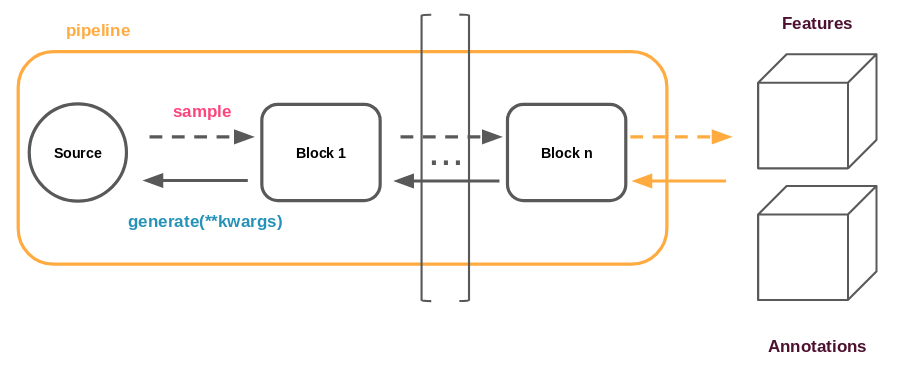
Among the existing blocks, there is one that is of particular interest to us: the one responsible for computing the features. It is instantiated from a configuration that contains a description of the features it should extract (there can be many when doing multi-modal learning for example).

On with our solution!

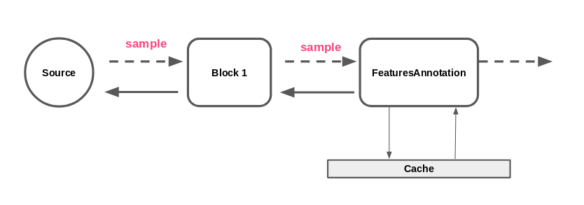
Without remote task distribution, we are find ourselves in the situation where a single FeaturesAnnotation block is used to compute features from a sample (possibly using multiprocessing).

The architecture we would like to reach is the following.

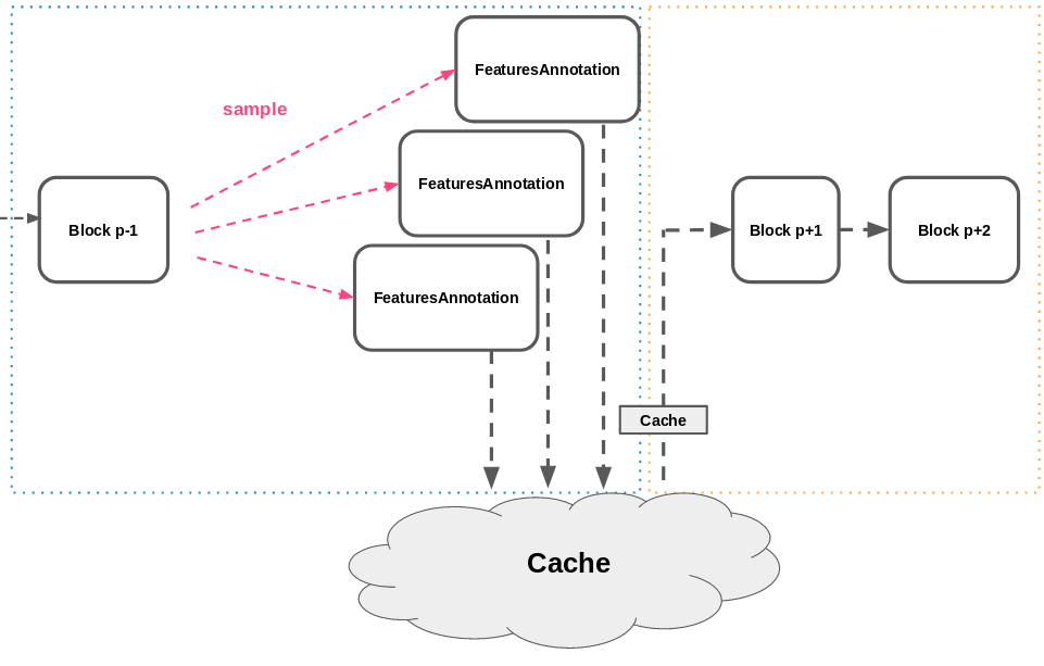
For simplicity and without any substantial incurring costs, we can imagine first computing offline all the features and store them into a cache. The features computation is split across many machines and the results are written to a shared cache. In our situation, the cache is shared by being written to an NFS.

This cache can then be copied locally to the machine that will run the experiment to reduce the read-times. When re-running the pipeline for training, the features computation step will have been reduced to a disk read.

Now that we have an idea of what we want to achieve, let’s move on to the implementation part!

Implementation

By now, we’re in the situation where we want to distribute a finite list of tasks to be handled by a cohort of workers. We want to be able to publish feature computation tasks associated with an experiment, and we want these tasks to be collected by workers. In terms of interface, we want to be able to interact with the system through a simple HTTP API, where we could post the configuration describing the experiment that we already use to train our models, and the features would start being computed in a distributed fashion.

Distributing

Quite a lot of solutions are available to perform the actual distribution of tasks. To reduce the field of possibilities, a few more requirements are worth mentioning:

• We want guarantees that all the tasks in the experiment are executed (no loss)
• We want the task queue to be persistent, so computation can be easily resumed in case of a failure
• The tasks taking a while to be executed, the publish rate for the tasks will never be a bottleneck. So we do not mind trading speed for robustness, or coding time.
• The implementation must not depend on the number of workers, and in particular, the number of worker must be flexible (with machines going offline, or new machines joining the work pool).

Put like this, it immediately calls to a centralized system, built around a broker. The broker would take care of the communication between publishers and workers, by receiving tasks, storing them to a queue, and handing them to workers that ask for it, while keeping tracks of the state the tasks are in.

All of this is done extremely well by RabbitMQ.

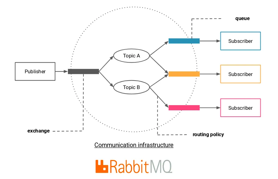
An advantage of going with RabbitMQ (over some other message brokers), is that there exists a very nice python framework called Celery, that provides an additional application layer over messaging protocols like AMQP (the one used by RabbitMQ), and which would make the development of our application considerably easier since it already implements the notions of task, publisher, worker, result back-end, removing the need to master the AMQP protocol.

Publishing and executing tasks is made really simple, all we have to do is the following.

From the publishers’ perspective:

• build a pipeline up to the FeaturesAnnotation block
• run it to get samples
• serialize these samples
• publish them as celery tasks

From the worker’s perspective:

• retrieve the configuration for the experiment
• instantiate the FeaturesAnnotation block
• start receiving samples
• run the features extraction on them (which comprises the caching to the shared cache)

Assimilating a Celery task message to a sample is an elegant solution because it eliminates “by definition” of the sample a lot of redundant information, and therefore keeps the network usage to a minimum. For example, the configuration describing the features to extract, common to all the samples, is only transmitted once to initialize the worker.

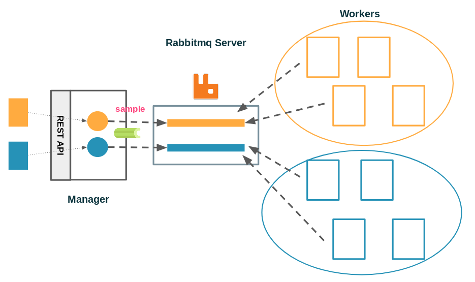
Zoom on the manager

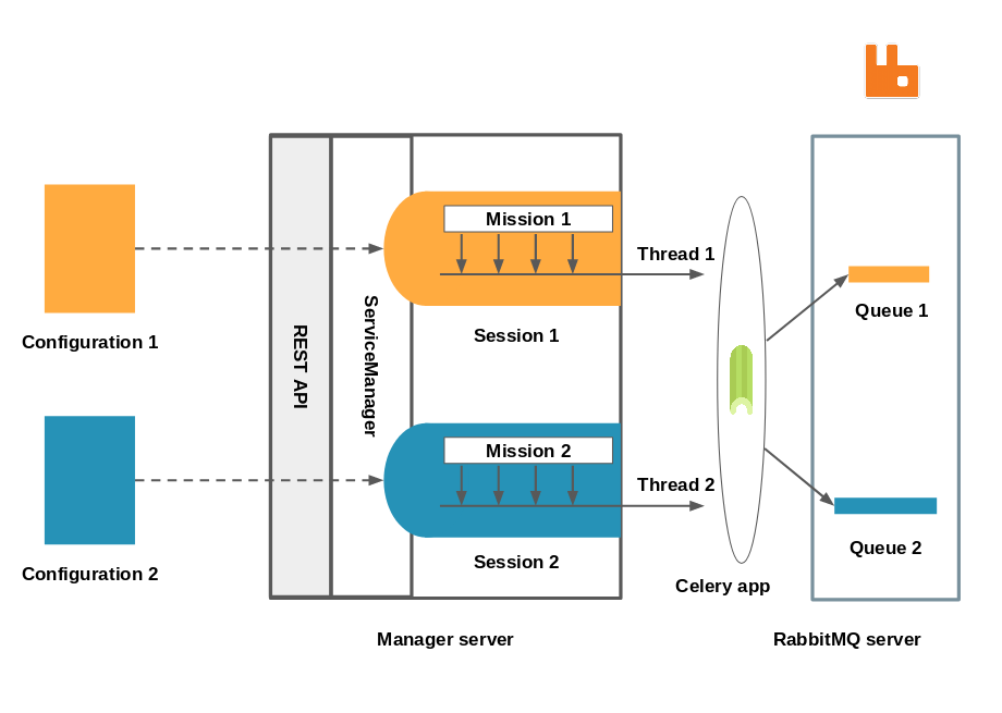
We have reached a state where we have a manager server, that exposes an API to which configurations for an experiment can be posted and handled by the service manager. The service manager is responsible for launching new computation sessions and administrating them. It holds references to all the sessions that are currently running. Each session is responsible for creating the exchange and the queue associated with it, and for publishing samples (or tasks) to it. The routing logic is extremely simple since there is a one to one mapping between an experiment and a queue, all of which are identified by a name. The worker only has to subscribe to a single topic and start consuming tasks from the corresponding queue.

A Celery application being thread safe, all the sessions’ publishing job are run in separate threads.

Controlling the publishing rate of the tasks

All of this works pretty well except on one point. The session can publish tasks at a much faster rate than the worker can consume them, which bloats up the queue. This is undesirable for many reasons, the most obvious being that we don’t want to saturate the rabbitmq server’s memory, which is a real risk especially when running many sessions at the same time.

Therefore, we came up with another component in the system to tackle this issue: a program that can be run from any machine in the same network as the manager and the RabbitMQ server, and whose job is to perform control over the tasks’ publish rate. It collects health metrics retrieved either from the manager’s API, or from the RabbitMQ server, and takes a decision to increase or decrease the publish rate for a session. When the new publish rate is decided, a call is made to the manager’s API to set it in the corresponding session. This presents a lot of advantages like:

• Freeing the manager from having to do that itself so it can focus its resources on the API and the session management.
• Dynamically adapting the publish rate to the available computing power, if a machine goes offline or if we add new workers. We know that we always make the best of the available power.
• Prevents the message queue from getting too big.

To do that we could have opted for full blown solutions like Prometheus but we felt like it was an over-engineered option to our rather simple case.

Our solution is a single python script called “health” based on Tornado, here is how it works.

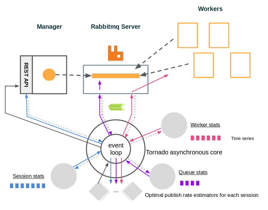
We have different monitors that periodically collect data asynchronously from the manager, the RabbitMQ server or the workers, and store these values in doubly linked list acting as time series. Values from these time series are also retrieved periodically through Tornado’s event loop by controller objects (one per session). These controllers use the retrieved data to make a decision as to how the publish rate should evolve, and send it to the manager.

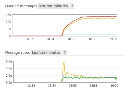
At this stage we have identified the different actors of the system and implemented what needed to be. Still, some questions remain: how to deploy all those bricks in practice, and in particular the workers? It is clearly out of question to run each of them manually.

Building a proper architecture for our system

Let’s containerize everything!

Now that we have carried the ground work, our application has individual parts that seem to get the job done. It is time to bring it all together and make the ensemble shine!

Enters Docker.

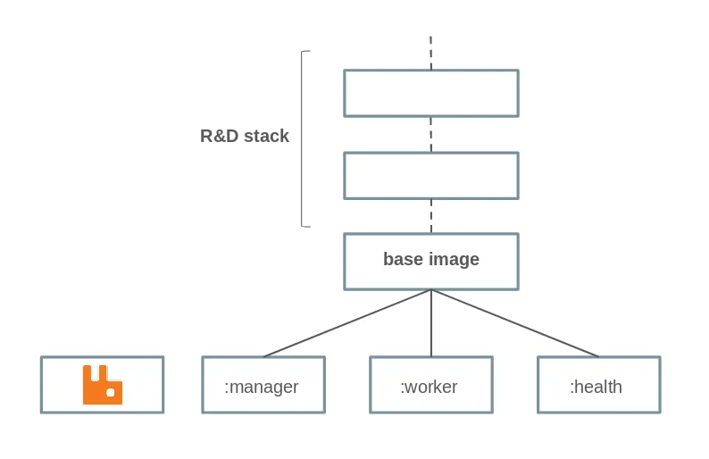
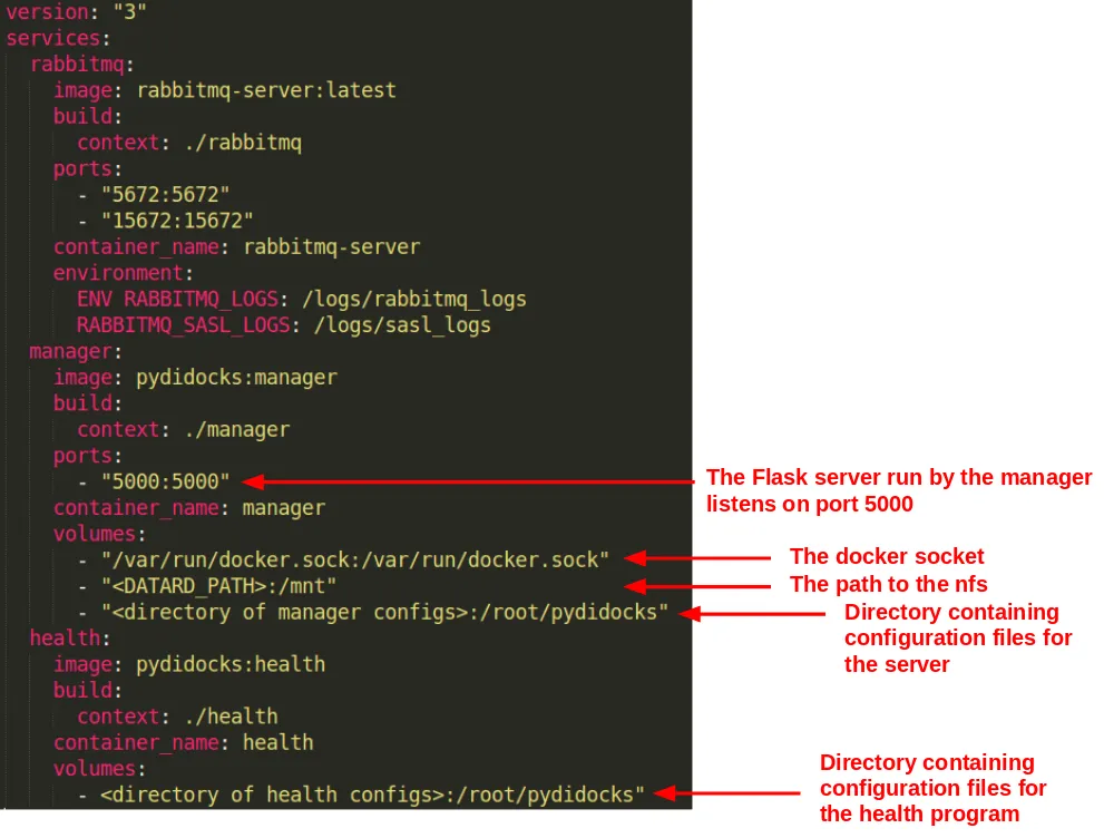
An advantage of the solution we have laid out, is that it is made of well separated actors behaving in a well defined environment. This makes the process of containerizing them a lot easier. When they are, we will be able to easily deploy the RabbitMQ server, the manager and the health program with docker compose. Deploying workers will just amount to creating a docker service.

By far the easiest part to containerize is the RabbitMQ server, because there is literally nothing to do! There is an official image for it so let us just use that. Actually, since we need the management plug-in, we deploy the image tagged “management”.

Here is the hierarchy of the docker images that we have built. Manager, worker and health mainly differ by the command run on launch.

Let’s deploy everything!

Now, deploying the Celery workers for an experiment becomes as simple as creating a swarm service. This is done by the Session objects using the docker-py module. It communicates with the Docker daemon on launch to create a service with the same name as the experiment.

The final strike

At this point, we are able to:

• Run all the components of the system with docker compose
• Create a swarm service to spawn Celery workers

There’s one glitch left to fix. Since the components need to be able to communicate with each other, the first thing we did was hard-code in the configuration files their addresses. This is clumsy since it requires us to change the address depending on the machine the components are running on. Now that we deploy with Docker Compose, all the components live in the same Docker network, and Docker takes care of resolving addresses from the component’s name! That means that instead of an explicit IP in our configurations we can use only “manager”, or “rabbitmq-server”.

Because the workers are deployed through docker swarm, and since they need to contact the manager to retrieve the configuration, it would be awesome to make sure they also belong to the same network in order to use the same trick and completely remove the need for any hard-coded IP.

When creating a service, it is possible to bind it to an existing overlay network. However, Docker Compose creates a bridge network by default. A simple solution to that is creating a specific network in the compose file. Another, is to deploy our components with docker stack. Docker stack will simply take the Compose file and use Swarm to deploy it. In doing so, it creates an overlay network, used by swarm, and now only remains to attach the services we create for this network.

We have now completely eradicated the need for any hard-coded address, and have robust way to deploy everything anywhere without any change, and docker stack can be used to update the software in one command!

docker stack deploy — compose-file docker/docker-compose.yml distributed_stack

We can now focus on the experiment ;).

Conclusion

We have described an architecture we have been using for a few months in production on our machines to process as quickly as possible all the computation task necessary to start the training of a deep learning experiment based on audio. How to easily deploy such architecture is a problem in itself for which we provided an answer that relies on powerful technologies like RabbitMQ and Docker (swarm and compose). Although we have deliberately chosen to present this work under the scope of our own activities (deep learning experiments), there is nothing so specific to deep learning in this architecture, and it should be suitable for a great variety of other use cases, where we simply wish to distribute a number of individual, independent tasks, in a processing pipeline.